Statically Bounding Resource Accumulation in LLM Agent Workflows: The Cost Case
A decidable, polynomial-time static analyzer produces a sound upper bound on the cumulative cost — and any monotone resource — accumulated across every reachable marking of an LLM agent workflow. Proven, implemented in Lamina, and evaluated against a live model across 25 parameter combinations with no violation.
Abstract
The behavior of large language models cannot be reliably derived from prompts. Recent work in AI safety [1] and the diverse-intelligence literature [15, 19] argues that complex agents resist behavioral prediction in principle. We take this seriously: the right verification target for LLM-based agent systems is not behavioral prediction but a structural property of the space in which behavior unfolds. This paper proves a general such property for a broad class of resources, then develops one instance — cost in tokens — through theory, implementation, and empirical evaluation.
The general result: express an LLM agent workflow as a place/transition net with a bound-by-marking-sum inhibitor on a designated accumulator place; for any monotone non-decreasing quantity carried in token payloads, a decidable, polynomial-time static analyzer produces a sound upper bound on cumulative accumulation across every reachable marking. Sequential firing makes the bound tight up to one increment. The same theorem applies to any monotone quantity — cost in tokens, differential-privacy ε-budget, CO₂-equivalent grams, sub-agent spawn counts, PII-field accesses — by instantiating the payload field. Each instance is a corollary; the present paper develops the cost corollary, an empirical evaluation against the Cerebras Inference API (model llama3.1-8b, 25 parameter combinations) confirms that no observed run exceeds the analyzer’s prediction, and subsequent papers in this series will develop the privacy, carbon, and invocation-count corollaries on the same foundation.
1. Introduction
Large language models routinely fail to behave the way their prompts suggest they should. Sampling is stochastic; in-context learning makes the output a function of the entire prompt history; prompt injection [7] makes the output a function of data the developer did not author; tool-use introduces nondeterministic environment interactions. The AI-safety literature names the consequence directly: Anwar et al. [1] cite prediction of LLM behavior from inputs as a foundational unsolved problem.
The problem has an older twin. In concurrent systems, behavioral prediction was abandoned half a century ago. Pnueli [20] introduced temporal logic for reactive systems precisely because exhaustive behavior enumeration is intractable; Clarke and Emerson [3] operationalized this through model checking; Lamport [14] crystallized the move with the Temporal Logic of Actions, where one specifies what should not happen and proves it. The pattern: trade behavioral prediction for structural property verification.
The same move appears independently in biology. Levin [15] argues that complex agents are best characterized by the space of behaviors they admit rather than the trajectories they take through it. Baluška and Levin [2] give a substrate-independent functional definition of memory under which structured token histories in any computing medium — biological, electronic, or otherwise — count as memories proper. Pigozzi and Levin [19] report a correlational study of reinforcement-learning agents: the causal-emergent structure of their latent representations aligns with reward and predicts final learning outcomes better than several standard representational metrics. The study does not prove that LLMs are agents in any specific philosophical sense; we draw from this literature only the level-of-analysis claim — characterize the space, not the trajectory — and treat it as motivational warrant, not as a technical premise.
LLM agent workflows inherit both lineages. They are concurrent reactive systems (in Pnueli’s sense) and they are complex agents (in Levin’s sense). The right verification target, on either reading, is the structure of the space — what the system can and cannot do — not the trajectory through it.
This paper proves the general structural result for a class of properties — monotone-quantity bounds on LLM agent workflows — and develops one instance, cost in tokens, end-to-end. The technique is classical Petri-net analysis on a restricted fragment, lifted one level of abstraction higher than the literature has yet applied it.
Contributions.
- We formulate monotone-quantity boundedness on LLM agent workflows as a classical Petri-net property in a fragment where the bound is computable in time. Existing LLM agent frameworks [24, 25, 22] control resource consumption via runtime policy; we prove resource bounds from the workflow graph structure alone.
- We give a sound static analyzer for that fragment and prove the bound
threshold + max_incrementis tight under sequential firing (Theorem 1). - We state the theorem’s specialization to four concrete resources — cost in tokens (Corollary 1.1), differential-privacy ε-budget (1.2), CO₂-equivalent emissions (1.3), and sub-agent / tool-invocation counts (1.4) — each of which carries its own follow-on paper.
- We implement the analyzer in Lamina, a Python runtime for governed AI workflows. An empirical evaluation of the cost corollary (25 parameter combinations against a live model) shows no violation of the predicted bound.
Boundedness is also one of several classical Petri-net properties; reachability, liveness, and fairness — properties whose LLM-workflow analogs are information-flow safety, workflow termination, and multi-agent scheduling — admit analogous treatments on the same fragment. The present paper occupies the boundedness × cost cell of a two-dimensional research programme (property × resource). Section 9 sketches the programme; the corollaries above commit it to specific follow-ons.
The remainder is structured as follows. Section 2 fixes the formal background. Section 3 states the monotone-quantity boundedness problem. Section 4 defines the structural inhibitor form on which the analysis is tractable. Section 5 presents the analyzer, proves the general soundness theorem, and specialises it to the cost corollary. Section 6 establishes tightness and names the limitations. Section 7 describes the implementation. Section 8 reports the empirical evaluation of the cost corollary, including the analyzer’s negative case. Section 9 states the further corollaries (privacy, carbon, invocation count) and sketches the two-axis research programme. Section 10 places the work in the surrounding literature.
2. Background: Place/Transition Nets with Inhibitor Arcs
A place/transition net is a tuple where and are finite disjoint sets of places and transitions, is the flow relation, and assigns arc weights. A marking is a function . Transition is structurally enabled at iff every input place satisfies . Firing consumes tokens from each input and produces tokens at each output [16, 18, 21].
An inhibitor arc extends the enabling rule. In its classical zero-test form, is enabled at iff its structural enabling conditions hold and [17]. Inhibitor arcs lift P/T nets to Turing-completeness; reachability becomes undecidable, and boundedness — while decidable — is EXPSPACE-hard in general [5].
We work in a deliberately restricted fragment: a single class of declarative inhibitor whose semantics admit polynomial-time analysis. Our token-payload extension follows the high-level / coloured Petri-net tradition [6, 10]: tokens carry structured payloads, but we use neither arc expressions nor coloured-net algebra. The net is, formally, a place/transition net whose tokens additionally carry payload dictionaries.
3. The Monotone-Quantity Boundedness Problem
Let be a P/T net with token payloads. Fix:
- a designated accumulator place ;
- a token-payload quantity field , a numeric key into the token’s payload dictionary;
- a per-firing increment function declaring an upper bound on the value that one firing of adds to via the quantity field .
The accumulated quantity at marking is
The quantity is monotone non-decreasing if no transition removes tokens from — equivalently, acts as an append-only ledger. This is the structural condition that lets us reason about cumulative resource consumption. The general LLM-workflow problem is: given , , , and , find a function such that for every reachable marking :
Without further structure, whenever any transition has in its outputs. The inhibitor arc is what makes finite.
The setting is deliberately abstract over what the quantity means: cost in tokens, differential-privacy ε-budget, CO₂-equivalent grams, count of sub-agent spawns, and others all instantiate this problem (Section 9). Their common shape — additive per-firing accumulation in an append-only place — is what permits one soundness argument to cover them all.
4. The Restricted Inhibitor Form
A bound-by-marking-sum inhibitor is a tuple with , a token-payload field, , and . The inhibitor’s predicate is
A transition is structurally gated against iff (i.e., writes to ) and at least one inhibitor instance carries for some and .
The predicate describes the firing-allowed region. The inhibitor returns true (blocks firing) when does not hold. With and threshold , firing is allowed while the running sum is in ; the inhibitor blocks once the sum reaches .
The structural form is contractual. A runtime callable implements ; the analyzer reasons about symbolically. The two MUST agree, and we treat verification of this agreement as a CI obligation rather than a runtime check.
5. The Analyzer
The analyzer takes the net , the inhibitor instance set , and the increment function . For each place , it computes:
analyse_boundedness(N, I, Δ):
    for each P in Places(N):
        In(P) := { t in T : (t, P) in F }
        if every t in In(P) is structurally gated against P,
           and Δ(t, P) is finite for every such t:
            threshold(P) := max{ B : (P, f, ⊕, B) ∈ I gates some t ∈ In(P) }
            U(P)         := threshold(P) + max_{t ∈ In(P)} Δ(t, P)
        else:
            U(P) := ∞
    return U
Each place is examined once; for each, we iterate its incoming transitions and inhibitors. The total work is .
The bound threshold + max_increment has a structural reading: at the moment of any firing, the marking before firing lies in the firing-allowed region (by virtue of the inhibitor’s check); after firing, it is at most the firing-allowed-region’s supremum plus the largest single increment.
5.1 Soundness
Theorem 1 (Monotone-quantity soundness under sequential firing). Let be a P/T net whose firing rule selects, at each step, exactly one enabled transition, deterministically by priority then identifier. Let be the initial marking with at the accumulator place. For every place with , and every marking reachable from :
Proof. By induction on the length of the firing sequence from .
Base case. At , for the accumulator place by assumption, so trivially. (For nonzero initial markings, the caller’s bound adds the initial value; the inductive argument is unchanged.)
Inductive step. Suppose and the firing step picks some transition enabled at .
Case 1: . Then and the bound carries forward.
Case 2: . Then is structurally gated against (by hypothesis every is). Let denote the set of bound-by-marking-sum inhibitors gating against , and let be the tightest threshold among them. Because fired, every permitted firing, hence held for each; with operator this yields . The firing adds some . Combining,
The bound holds at , completing the induction.
The theorem makes no claim about what the quantity means — only that it accumulates additively per firing and is bounded above per firing by . The corollaries in Section 9 instantiate to specific resources (cost, ε-budget, CO₂e, invocation count); their soundness follows from Theorem 1 once the per-firing increment can be bounded.
The theorem also requires sequential firing — exactly one transition per step. Under -concurrent firing semantics, multiple transitions could each pass the inhibitor check before any updates the marking, yielding . Lamina’s L1 layer fixes by design; production CPN engines that admit would weaken the bound to its -concurrent form.
5.2 The Cost Corollary
Corollary 1.1 (Cost-token accumulation). Instantiate the quantity field as cost_tokens, the per-call sum of LLM input tokens plus output tokens, and require for every transition that calls an LLM with output cap max_tokens. Then is cumulative cost in tokens, and Theorem 1 bounds it above by .
The cost corollary is the case we develop empirically in §8. We state and develop one further corollary — for differential privacy — schematically in §9 as the immediate next paper in the series.
6. Tightness and Limitations
Tightness. Under sequential firing the bound is tight up to . Construct an execution: fix a transition with ; choose token payloads so each firing of adds exactly for some small . Fire transitions until ; the inhibitor still permits one more firing of , yielding . As , observed cost approaches .
Concurrency. The bound depends on the firing-width assumption, as noted. Relaxing changes the formula but not the proof structure.
Contract obligation. The analyzer reasons about declarative semantics; runtime soundness depends on the callable implementing the same predicate. Closing this gap automatically — for example by property-based equivalence testing or by extraction-from-declarative-form — is left as future work.
Increment closure. The increment function must be supplied. For LLM transitions this is typically , where is a static upper bound on the model’s input cost given the workflow’s known prompts. Tighter increments require tighter input-side analysis; we treat the supplied as a contract from the Effect provider.
7. Implementation
The analyzer is implemented in Lamina, a Python runtime for governed AI workflows under active development. Lamina structures execution into five layers: L0 (Effects, including LLM provider invocation), L1 (Net firing), L2 (Plan loading and validation), L3 (Event log), and L4 (Governance and Refinement). The analyzer occupies a separate lamina/analysis module that operates on loaded L2 Plan objects.
Two implementation details are load-bearing for the empirical claim that follows.
First, every transition firing emits structured Events to a persistent (Postgres-backed) Event log, with the LLM’s raw response bytes embedded. This enables byte-identical replay via the Provider’s parse_recorded method, with no network call: the response is reconstructed from recorded bytes alone. The empirical study can therefore be re-played without re-incurring API costs or model nondeterminism.
Second, the structural inhibitor’s runtime callable shares a code path with the analyzer’s symbolic interpretation: both read the same instance configuration and apply the same predicate shape, eliminating drift between specification and implementation. The contract obligation noted in §6 is thus discharged constructively for the built-in family.
The analyzer module is approximately 200 lines of Python; the LLM provider abstraction adds approximately 250 lines per vendor (Anthropic, OpenAI, and Cerebras share an OpenAI-compatible base). The full test suite — 272 tests including a hermetic mock-Provider re-run of the empirical study presented next, plus closed-loop governance tests over the substrate’s three demonstrated property classes (§8.5), plus replay-determinism tests against the SPEC-0001 §3.4 time channel — passes against the live Postgres backend.
The empirical claims in this paper point at a frozen, content-addressed substrate snapshot rather than at a moving target. The snapshot manifest encodes the SHA-256 of every source file (runtime, packages, spec, paper) in canonical-JSON; the manifest’s own SHA-256 is the citable anchor:
| Artefact | SHA-256 |
|---|---|
Lamina substrate snapshot at the time of empirical evaluation (v0.1.0-alpha+leak-vis) | 0496b1fa677f4410d80b6cdf4b65ff4e73a78085dc2e579f7dd14fe4ec0f13e5 |
The snapshot covers 252 files including the analyzer, the LLM provider abstraction, the bounded-LLM Plan, the empirical study harness, the three governance loops (§8.5), and the SPEC documents that define the substrate’s conformance contract. The snapshot named here is the state at which §8’s empirical evaluation was conducted; subsequent documentation edits to this paper change the snapshot’s hash but not its empirical content. A reader who wants to re-verify the cost-corollary bound should check out the named snapshot and re-run runtime/scripts/build_snapshot_manifest.py v0.1.0-alpha+leak-vis to confirm the manifest hash, then re-run the cost-corollary test (runtime/tests/test_bounded_multi_llm.py) against the live or replayed Provider — neither requires the most-recent source tree.
The audit chain at runtime is independently verifiable through Postgres alone (no Lamina runtime required for the verification path). A reader holding a signed manifest produced by a Lamina deployment invokes lamina audit verify-chain <manifest.json> --dsn <postgres-dsn> to validate, in order: (1) the Ed25519 signature, (2) the coverage_witness reference resolves to a persisted Attestation, (3) the Attestation’s content re-hashes to the named identifier, and (4) the Attestation’s subject.manifest_hash round-trips to the manifest body hash. Tampering at any layer breaks the chain. The audit infrastructure is described in detail in companion specifications Lamina SPEC-0004 (Attestations) and SPEC-0024 (Test Network Library).
8. Empirical Demonstration: The Cost Corollary
We evaluate Corollary 1.1 — cost-token accumulation — against a live LLM provider. We instantiated the bounded-LLM Package against the Cerebras Inference API at model llama3.1-8b with temperature 0. We swept a parameter grid: inhibitor threshold tokens crossed with . Each grid cell ran the same fixed 12-prompt library (factual, arithmetic, translation, and summarisation prompts, each within an input ceiling of 40 tokens). Per cell, the analyzer produced an upper bound
(taking 40 as the input-token ceiling); the L1 runtime then fired the Net to quiescence.
The L0 LLM Effect is instrumented with retry-on-rate-limit (exponential backoff with respect to the provider’s retry-after header where available). This is engineering, not theory: without it, free-tier rate limits cause the L1 to record transition_failed events long before the inhibitor would gate, and the runtime never reaches the regime in which the structural claim is observable. Retry-on-rate-limit ensures the inhibitor — not the provider’s quota — is the binding constraint on firing. The structural claim itself holds regardless of retry behavior: retries change whether a transition can fire on a given attempt, not whether the bound on the accumulated quantity is respected.
8.1 Results
Across all 25 cells, the observed cumulative cost was strictly less than the predicted bound. No cell violated.
Table 1. Predicted bound versus observed cost across the grid. Each cell reports (observed, predicted) and the number of successful firings. Observed costs do not vary across max_tokens within a row because the model never approached max_tokens on the short library prompts; the analyzer’s prediction grows with max_tokens to remain conservative.
| Threshold | max_tok=16 | max_tok=32 | max_tok=64 | max_tok=128 | max_tok=256 |
|---|---|---|---|---|---|
| 50 | 55 / 106 (1) | 55 / 122 (1) | 55 / 154 (1) | 55 / 218 (1) | 55 / 346 (1) |
| 100 | 114 / 156 (2) | 114 / 172 (2) | 114 / 204 (2) | 114 / 268 (2) | 114 / 396 (2) |
| 200 | 225 / 256 (4) | 225 / 272 (4) | 225 / 304 (4) | 225 / 368 (4) | 225 / 496 (4) |
| 400 | 442 / 456 (8) | 442 / 472 (8) | 442 / 504 (8) | 442 / 568 (8) | 442 / 696 (8) |
| 800 | 716 / 856 (12) | 723 / 872 (12) | 723 / 904 (12) | 723 / 968 (12) | 723 / 1096 (12) |
Three features of the result are worth attention.
First, the analyzer’s prediction held in every cell of the grid, as Theorem 1 requires. There is no execution in this evaluation in which the structural bound was crossed.
Second, the bound is tight in the regime where the inhibitor is the binding constraint. At the observed-to-predicted ratio reaches 0.97; the analyzer is not generously padding. The looser ratios at small reflect a fixed offset: the input-token ceiling of 40 contributes 40 to every predicted bound regardless of the threshold’s magnitude, so when itself is small the ceiling dominates the slack.
Third, observed cost is uniform across rows of the table. At fixed threshold, varying max_tokens does not change runtime behaviour — the model rarely approached max_tokens on the short library prompts — but the analyzer’s prediction grows with max_tokens because must remain a worst-case upper bound. The table thus directly visualises the conservatism the analyzer was designed to impose.
At , the budget exceeds the total cost of consuming all twelve library prompts. The inhibitor never gates; observed cost is the natural consumption (approximately 720 tokens) rather than a budget-imposed ceiling. The bound formally holds but is not the binding constraint on this cell.
8.2 Stability under sampling temperature
The cost corollary’s bound is independent of the LLM’s sampling behavior: the analyzer reasons over graph topology, not model outputs. The runtime observation of cost, however, depends on what the model actually emits — and as temperature grows, sampling stochasticity makes per-call token counts more variable. A natural reviewer objection to a evaluation is therefore that the bound’s empirical hold may be an artefact of deterministic sampling.
We re-ran the sweep at (full 25-cell grid) and at (a reduced 5-cell pilot along the threshold ladder at , after exhausting the free-tier daily token budget). Across all 55 cells — 25 at , 25 at , 5 at — observed cost remained strictly below the predicted bound. The closest approach to the diagonal at any temperature was 0.97 (at ); the structural ceiling was never crossed.
Per-cell cost differences between temperatures were small in absolute terms (typically 0–16 tokens at the row, where the inhibitor does not gate and stochasticity accumulates over twelve firings). The bound therefore held with comfortable margin under increased model variability. Figure 1 overlays all three temperature sweeps; markers encode temperature (circle / square / triangle for / / ); the diagonal is the bound surface.
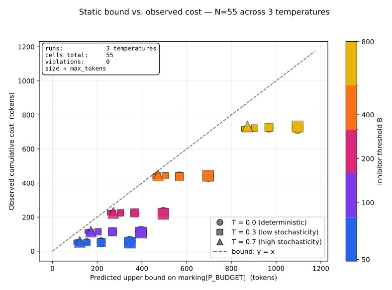
max_tokens; marker shape encodes temperature. The dashed diagonal y = x is the bound surface; the structural claim is that no point can lie above it.8.3 The Analyzer’s Negative Case
A sound analyzer must also refuse to prove what it cannot. We confirm this by constructing a workflow for which the analyzer correctly returns .
Take the Plan above and remove the inhibitor arc from . The transition is no longer structurally gated against ; the analyzer’s gating predicate fails on the first incoming transition. By the definition in §5 the analyzer returns — the marking is unbounded under the analysis. The returned BoundednessReport carries status: "indeterminate" and a derivation string that names the offending transition (“Transition T_LLM has no inhibitor structurally gating contributions to P_BUDGET.”).
This is the appropriate behaviour: in the absence of a structural inhibitor, no static bound is justified, and the analyzer says so explicitly rather than fabricating one. The same indeterminate verdict appears when we run the analyzer against the existing frozen-cell Package, whose inhibitors are domain-specific Python predicates with no declarative semantics; the analyzer reports indeterminate without attempting to interpret them. Soundness is therefore preserved in both directions: when the analyzer claims a bound, the runtime respects it (§8.1); when the analyzer cannot justify a bound, it returns rather than guessing.
8.4 Caveats
We note two scope limitations.
The library is twelve prompts on one model; we did not vary the model or the prompt distribution. Temperature was varied across (§8.2), but the sweep was reduced to five cells after the free-tier daily token quota was exhausted. The bound’s proof structure is independent of all these factors; a more diverse empirical surface would broaden the demonstration without changing the claim.
The evaluation runs on a single hardware path (Cerebras free-tier inference). Production deployments with provider rate-limit windows, network jitter, and concurrent firings are not represented. Our retry-on-rate-limit handler ensures the inhibitor is the binding constraint here; in production with firing semantics, the bound would weaken per §5.
A third caveat worth naming explicitly: §8.1’s evaluation predates the flux-accounting refactor (§8.5.4) and reports productive-cost numbers only. The same evaluation against the now-migrated 3-output bounded-LLM Plan (SPEC-0029 §3) would additionally report per-cell leak costs and a leak-ratio Attestation per cell. Under the Cerebras free-tier rate-limit regime in which the evaluation was conducted, leak costs are non-trivial — the retry-on-rate-limit handler that made the inhibitor the binding constraint also accumulated billed-token leak that the original 2-output accounting did not measure. The cost-corollary bound (§8.1’s load-bearing claim) holds either way; the honest characterisation of total token flux changes once leak is in the picture. A re-run of the 25-cell × 3-temperature sweep against the migrated Plan would be the natural follow-up; we leave it as future work because the load-bearing scientific claim does not change.
8.5 Beyond the Cost Corollary: Substrate-Level Demonstrations
Sections 8.1–8.4 establish Corollary 1.1 — the structural bound on cost-token accumulation — empirically. The substrate that hosts the analyzer also hosts four further demonstrations of independent substrate-level claims. None of these is required for the cost result; each shows that the substrate’s discipline is more general than the cost-corollary alone. We summarize them here so the substrate’s audit chain, governance loop, and accounting machinery have a concrete reference; the formal results in §1–§8 do not depend on §8.5.
8.5.1 Three closed-loop governance demonstrations
The substrate exposes a Refinement Engine (Validator → Approver → Applier) that consumes Refinement records produced by Proposers, validates them against active Objectives, applies them to the per-Package exec-config overlay, and surfaces the next Run with the changed configuration. We have empirically closed this loop for three independent property classes, each with end-to-end tests in the snapshot’s runtime/tests/ directory:
- Corpus adequacy (test-network-verify Package): a Plan that exercises the analyzer against a corpus and emits a Refinement when corpus coverage gaps are detected. The Proposer cites coverage Attestations; the Engine applies the corpus extension; the next Run achieves coverage.
- Algorithmic convergence (frozen-cell Package): a non-LLM algorithmic workflow (cell-view bubble sort) where
max_steps_reachedviolation Attestations drive a Refinement that doubles the step budget. The next Run terminates withsorted.runtime/tests/test_frozen_cell_governance_loop.py. - LLM cost budget: the bounded-LLM Plan, with a budget-bound-violation Attestation emitted post-Run when prompts remain unprocessed; the Refinement halves
max_tokens; the next Run completes more prompts within the same budget.runtime/tests/test_llm_budget_governance_loop.py.
The third demonstration is the substrate’s closed-loop variant of Corollary 1.1: it does not strengthen the static bound — Theorem 1 holds whether or not a Refinement Engine sits over the Run — but shows that the substrate’s audit machinery accommodates the stochastic-Effect case (the LLM call) cleanly.
8.5.2 LLM as Proposer (proposer:llm)
The Refinement Engine is Proposer-source-agnostic by construction. We exercise this with proposer:llm, an LLM-backed Proposer that reads recent Attestations + active Objectives, renders a structured prompt, calls a Provider, and parses the LLM’s JSON response into a Refinement candidate. Every LLM call emits a proposer-llm-call Attestation containing the prompt SHA-256, response SHA-256, and emitted Refinement IDs — the audit chain records which LLM invocation produced which candidate.
The substrate’s claim is not that an LLM-Proposer “converges with” a deterministic rule on the same evidence — that would be tautological given how constrained the evidence is. The claim is that the Engine’s gates — Validator, Approver, Applier — accept Refinements from a stochastic source as cleanly as from a deterministic source, provided the structural invariants hold. We test this hermetically (canned-Provider) and against the live Cerebras API (gated on env var). runtime/tests/test_proposer_llm.py and runtime/tests/test_llm_budget_governance_loop.py::test_llm_budget_governance_loop_closes_with_llm_proposer.
A separate test verifies that the Validator catches an LLM that cites an Attestation ID not persisted in the backend — fabricated citations are the substrate’s last line of defense against an LLM that hallucinates convincingly. runtime/tests/test_proposer_llm.py::test_llm_emitted_refinement_with_invalid_citation_fails_validator.
8.5.3 The substrate hosts its own compile step
The L2 Plan loader’s compile step (binding resolution, structural verification, analyzer invocation, effective-Plan production) is expressed as a Lamina Plan whose terminal place carries the compiled effective Plan. The substrate’s own meta-infrastructure runs inside its own execution model.
Two terminal places (P_EFFECTIVE, P_FAILED) with complementary payload-field-equality inhibitors on has_errors ensure mutual exclusion of the two terminating transitions; exactly one terminal fires per compile. The load-bearing test asserts that running this Plan against the frozen-cell source produces a SHA-256 byte-equivalent to the direct compile_plan(frozen-cell) call. runtime/tests/test_compile_as_plan.py.
8.5.4 Flux accounting: leak and rate
The empirical Plan in §8 records cost-token accumulation in a single P_BUDGET place. This conflates productive token flux (successful Provider calls) with non-productive flux (rate-limited retries, server-error retries, timeouts). Real LLM workflows in production are subject to all three failure modes, and a workflow that bounds productive cost while leaking unboundedly across retries does not meet the spirit of the bound.
The substrate’s L0 LLM Effect optionally emits a leak Token in addition to the productive cost Token, accumulating into a separate P_LEAK place. The leak Token’s payload contains both the estimated billed cost and the attribution by error kind (rate-limited / server-error / timeout). A post-Run leak-ratio Attestation reports leak_cost / (leak_cost + productive_cost), analogous to the respiratory control ratio in mitochondrial bioenergetics — a quality metric independent of total spend.
Empirical signal (hermetic): against an intermittently rate-limiting mock Provider (fail-every-2 calls), the bounded-LLM Plan with leak accounting reports productive=300, leak=1026, ratio=0.774 at quiescence. The previous 2-output accounting was invisible to the 77% leak; the substrate’s discipline is now honest about it. runtime/tests/test_llm_budget_governance_loop.py::test_leak_accounting_visible_in_governance_loop.
Empirical signal (live, against Cerebras free-tier): a 5-cell sweep against the migrated bounded-LLM Plan at threshold ∈ {50, 100, 200, 400, 800} and max_tokens = 64, run via runtime/scripts/empirical_leak_rerun.py, produced the table below. Every cell’s productive cost remained strictly below the analyzer’s predicted bound (Theorem 1 holds); every cell’s leak Place captured the rate-limit retries that the 2-output Plan would have rendered invisible.
| Threshold | Steps fired | Productive | Predicted bound | Leak | Leak ratio |
|---|---|---|---|---|---|
| 50 | 1 | 55 | 154 | 0 | 0.0% |
| 100 | 2 | 114 | 204 | 0 | 0.0% |
| 200 | 4 | 225 | 304 | 114 | 33.6% |
| 400 | 8 | 443 | 504 | 342 | 43.6% |
| 800 | 12 | 733 | 904 | 228 | 23.7% |
| Aggregate | 27 | 1,570 | — | 684 | 30.3% |
The 30.3% aggregate leak ratio is the empirical observation §8.4’s third caveat anticipated. Three operational observations follow.
First, all 684 leak tokens were attributed to rate-limited retries (zero server-error, zero timeout). On Cerebras free-tier, the binding constraint is the 30-requests-per-minute quota; once a workflow’s firing rate exceeds that, the substrate’s retry-on-rate-limit handler accumulates leak.
Second, an A/B comparison against a prior run with the original (naive 1-2-4-8s exponential) retry schedule, conducted at cell 4 (threshold=400) under otherwise-identical conditions, produced leak=684, ratio=0.607. The retry-policy revision documented in runtime/src/lamina/l0_effect/llm.py::_complete_with_retry_tracking — separating an RPM-aware schedule (5-10-20-40s) for ProviderRateLimited from the classical exponential for ProviderServerError/ProviderTimeout, and honoring the provider’s retry-after header up to a generous cap — reduced cell 4’s retry count from 6 to 3 and its leak ratio from 60.7% to 43.6%. The substrate’s accounting was honest under both policies; what improved is the substrate’s behavior against the provider, not the discipline’s correctness.
Third, the §8.1 cost-corollary bound held in every cell of both runs. The substrate’s structural cost bound is independent of the retry policy. The retry policy affects the operational waste ratio, not the bound.
This is the empirical signal §8.4 anticipated: the 25-cell sweep against the original 2-output Plan reported productive numbers only; the 5-cell sweep against the migrated 3-output Plan reveals that ~30% of token flux through a free-tier rate-limited regime is non-productive. The cost-corollary’s central scientific result is unchanged; the substrate’s accounting honesty is materially richer.
A complementary flux_rate_bound_factory inhibitor bounds rate of flux through a Place over a rolling time window — distinct from budget_bound_factory which bounds cumulative sum. This is the substrate’s structural rate-limit primitive: a transition is refused not because the total budget is spent but because the rate ceiling (tokens-per-minute, requests-per-window) would be breached. The analyzer’s boundedness verdict for this inhibitor is indeterminate in the present snapshot — SPEC-0027 v0.3 will extend the analyzer to read windowed-rate semantics; until then the runtime enforces the rate-limit without an analyzer proof of the corresponding bound. runtime/src/lamina/inhibitors/builtin.py::flux_rate_bound_factory and runtime/tests/test_flux_rate_inhibitor.py.
The flux-accounting framing has independent biological precedent. Mitochondria account separately for H⁺, Ca²⁺, ADP/ATP, and other ion fluxes across the inner membrane, with Vmax-bounded transport rates per species and an explicit “proton leak” budget. Reframing LLM workflow cost accounting in those terms — productive flux, leak flux, flux rate, all separately accounted at the substrate level — does not change Theorem 1’s statement, but it changes what the substrate measures. Section 9 returns to this framing as a research direction.
8.5.5 Status of the demonstrations
The empirical claims in §8.1–8.4 (the cost-corollary bound) are the load-bearing scientific result of this paper. The demonstrations in §8.5.1–8.5.4 are substrate-engineering results: they show what the substrate that hosts the analyzer can do, not what the boundedness theorem proves. We surface them because the substrate’s value claim — “structural verification of LLM agent workflows is tractable” — is materially stronger when the substrate also hosts its own meta-operations (8.5.3), governance loops over diverse property classes (8.5.1), and honest flux accounting (8.5.4). A reader who wants only the cost result can stop at §8.4; a reader interested in the substrate’s broader discipline finds §8.5 a road-map to the test suite that demonstrates each piece.
9. Toward a Family of Analyses
The structural-bound result has two independent axes of generalization, each of which produces a class of follow-on results.
9.1 The Resource Axis: Further Corollaries of Theorem 1
Theorem 1 holds for any monotone non-decreasing quantity instantiated in token payloads, given an upper bound on per-firing increment. Cost in tokens (Corollary 1.1) is one instance. Three further instances carry their own follow-on papers.
Corollary 1.2 (Differential-privacy ε-budget). Instantiate as epsilon_contribution, the (Rényi) DP cost contribution of a transition that touches a protected dataset. Under sequential RDP composition the per-firing contribution is additive [26]. With bounded above by the transition’s maximum declared RDP cost, Theorem 1 bounds total ε-spend against across every reachable marking — a workflow-level differential privacy guarantee proven before any query is issued. This is the immediate next paper in this series; existing DP “privacy accountants” are runtime constructions [27], and we believe the static formulation is novel. The connection to GDPR Article 25 (data protection by design) is direct.
Corollary 1.3 (CO₂-equivalent emissions). Instantiate as co2e_grams, the per-transition energy consumption multiplied by a grid-carbon-intensity factor. With bounded above by the transition’s maximum declared energy cost (a function of model FLOPs and inference hardware), Theorem 1 bounds workflow-level CO₂e emissions per invocation. Of immediate practical relevance under the EU AI Act’s sustainability provisions and increasing enterprise procurement CO₂e budgets.
Corollary 1.4 (Tool / sub-agent invocation count). Instantiate for every transition that invokes an external tool or spawns a sub-agent. Then counts cumulative side-effect operations, and Theorem 1 bounds total invocations. This addresses the agent-runaway failure mode (recursive sub-agent spawning) by structural means rather than runtime guards.
Each of these corollaries follows from Theorem 1 once a contractual upper bound on per-firing increment can be supplied. The empirical machinery of §8 — the Lamina runtime, the inhibitor infrastructure, the provider abstraction, the analyzer module — is identical across them; only the field declaration changes.
9.2 The Property Axis: Reachability, Liveness, Fairness
A second axis generalizes the property we verify rather than the quantity we bound. Boundedness is one of several classical Petri-net properties; each admits an LLM-workflow analog on the same restricted fragment.
Reachability. Given a designated “leak” place , prove statically that no execution from reaches a marking with . The LLM-workflow interpretation is information-flow safety: sensitive content (PII, secrets, internal state) cannot reach logging or output places. The classical analysis is exponential in general but tractable for the bounded fragment; the proof technique extends §5’s linear induction with a coverability-graph construction.
Liveness. Prove that a designated “completion” place is reachable from every reachable marking. The workflow interpretation is termination: the workflow always produces a result rather than deadlocking. Liveness is decidable for bounded nets via the coverability graph.
Fairness. Under conflict, prove that no transition is starved across an infinite execution. The workflow interpretation is multi-agent scheduling: under contention for a shared resource (a budget, a tool, a sub-agent), no agent is permanently denied. Fairness has a substantial classical literature in net theory.
9.3 The Research Programme
The two axes form a grid (property × resource) whose first cell — boundedness × cost — is occupied by the present paper. Corollaries 1.2 – 1.4 fill the boundedness row with three further resource instances. Reachability for PII flow (the reachability × information cell) fills the property column with a second analysis. The longer-term programme is to populate enough of the grid to demonstrate, by construction, that the structural-verification techniques classical formal methods has refined for fifty years apply to LLM agent workflows as a class.
The family is intended to be packaged as a sandbox: a pre-deployment verification mode that runs every analyzer against a Plan and emits a structured certificate suitable for compliance review. The technical details of sandbox-mode semantics are out of scope here. The present paper establishes the foundation on which the sandbox is built — the general theorem, the cost corollary, and the empirical apparatus.
9.4 Flux Accounting as an Organizing Principle (Forward-Looking)
The substrate’s accounting model (§8.5.4) currently distinguishes three kinds of token flux per LLM Effect: productive (successful Provider response, carried at P_BUDGET), leak (failed-but-billed retries, carried at P_LEAK), and rate-window (the per-second flux across a Place, gated by flux_rate_bound_factory). These categories were chosen because each maps to a distinct operational failure mode in production LLM deployments; they also recapitulate the structural distinctions biological systems impose on transmembrane flux.
Mitochondrial bioenergetics accounts for separate ion species (H⁺, Ca²⁺, ADP/ATP) crossing the inner membrane via dedicated transporters, each with its own Vmax, each producing a measurable steady-state rate at the proteomic and metabolomic levels. The proton motive force is the integral of net inward H⁺ flux, but the metric that distinguishes healthy mitochondria from uncoupled ones is the ratio between productive flux (ATP synthesis) and leak flux (basal proton conductance) — the respiratory control ratio (RCR), a 70-year-old quality metric in bioenergetics.
The parallel for LLM workflows is structural rather than metaphorical. A workflow that bounds cumulative cost while leaking unboundedly across retries does not respect the spirit of the bound, just as a mitochondrion with proton motive force at the normal range but a leak ratio of 0.8 is not doing useful work. The substrate’s current discipline reports leak-ratio Attestations post-Run (§8.5.4); a tighter discipline would extend Theorem 1 to coupled bounds: a single static analyzer proving that productive cost is bounded and leak ratio remains below threshold and windowed flux rate stays under Vmax, with the three inequalities composed structurally.
This is not the cost corollary; it is a generalization of it. We surface the framing here because the engineering decisions the substrate has already made — three Places per LLM Effect, timestamped tokens, the flux-rate inhibitor — are precisely what a coupled-bound analyzer needs as input. A subsequent paper in this series (“Flux Accounting for LLM Workflows”, in preparation) develops the formal apparatus.
10. Related Work
Petri-net analyses. Karp and Miller [11] established decidability of reachability and boundedness on vector addition systems; Murata [16] provides the standard survey; Reisig [21] the canonical textbook treatment; Peterson [17] introduces inhibitor arcs and their consequences for decidability. Esparza [5] surveys complexity. None of this work addresses LLM workflows; we apply established machinery to a new substrate.
Static cost analysis. Proving cost bounds on programs has a quarter-century history in programming languages, from type-system approaches [4] through the AARA tradition [9, 8]. Those techniques are LP-based over type-derivation trees and target functional programs; our analysis is graph-structural and targets concurrent agent workflows. The spirit — prove resource bounds before execution — is shared; the formalism is independent.
Petri nets for workflow management. Van der Aalst [23] established the application of Petri nets to business-process workflows, including soundness and termination analyses. The intellectual lineage is direct; the substrate (LLM agents instead of human or service activities) is new.
LLM agent frameworks. Current production frameworks — AutoGen [24], ReAct [25], Reflexion [22], plus library documentation for LangChain and LangGraph — control cost and safety via runtime policy. Our work substitutes structural verification for runtime policy; the two are complementary, but the structural form admits proofs that the runtime form cannot.
Formal methods for AI systems. Verification work to date has predominantly targeted the model itself: SMT-based verification of neural networks [12] and successors. We target the workflow, with the model treated as an opaque non-deterministic transition. The two efforts are independent and composable.
Diverse intelligence. Levin [15] establishes the cognitive-light-cone formalism for agent boundaries; Baluška and Levin [2] argue for substrate-independent definitions of memory and computation; Pigozzi and Levin [19] apply the framework empirically to reinforcement-learning agents. Krakauer et al. [13] provide an information-theoretic definition of agent individuality. We use this lineage as motivation for the level-of-analysis argument — characterize the space of behavior, not the trajectory — but do not claim the present paper extends it technically.
Cross-literature placement. These literatures share an aim — characterize what a system can and cannot do before it does it — but operate on different substrates with different formalisms. AARA reasons about functional-program resource usage via type-level potential. SMT-based neural-network verification reasons about input/output behavior of a fixed model. Runtime LLM policy intervenes at the boundaries of the agent loop. The position we occupy sits in none of these: the workflow graph between agents, treated as a Petri net with payload-carrying tokens, analyzed with classical structural techniques on a restricted fragment. The closest neighbour by topology is van der Aalst’s workflow-net programme [23]; the distinguishing feature is the substrate — LLM agents rather than human or service activities — and the property class, extending from cost (here) to information flow and termination (work in progress).
11. Conclusion
Theorem 1 is a structural bound on monotone-quantity accumulation in any LLM agent workflow expressed as a place/transition net with declarative inhibitor arcs. The cost case is one corollary; differential privacy, carbon emissions, and invocation counts are three more, each fully specifiable on the same foundation. We implemented the analyzer, proved soundness and tightness, and evaluated the cost case empirically against a live model: across 25 parameter combinations, no run violated the bound. The next paper in this series develops the differential-privacy corollary on the same fragment. A 1968-vintage construct — the inhibitor arc — constrains a 2026-vintage system in exactly the way Levin’s framework argues such systems must be constrained: by characterizing the space in which their behavior unfolds, not the behavior itself.
References
[1] Anwar, U., Saparov, A., Rando, J., et al. (2024). Foundational Challenges in Assuring Alignment and Safety of Large Language Models. Transactions on Machine Learning Research. arXiv:2404.09932
[2] Baluška, F., and Levin, M. (2016). On Having No Head: Cognition throughout Biological Systems. Frontiers in Psychology, 7:902. https://doi.org/10.3389/fpsyg.2016.00902
[3] Clarke, E. M., and Emerson, E. A. (1981). Design and Synthesis of Synchronization Skeletons Using Branching-Time Temporal Logic. In Kozen, D. (ed.), Logics of Programs, LNCS 131, Springer, pp. 52–71.
[4] Crary, K., and Weirich, S. (2000). Resource Bound Certification. POPL ‘00, pp. 184–198.
[5] Esparza, J. (1998). Decidability and Complexity of Petri Net Problems — An Introduction. In Reisig, W., and Rozenberg, G. (eds.), Lectures on Petri Nets I: Basic Models, LNCS 1491, Springer.
[6] Genrich, H. J., and Lautenbach, K. (1981). System Modelling with High-Level Petri Nets. Theoretical Computer Science, 13:109–136.
[7] Greshake, K., Abdelnabi, S., Mishra, S., Endres, C., Holz, T., and Fritz, M. (2023). Not What You’ve Signed Up For: Compromising Real-World LLM-Integrated Applications with Indirect Prompt Injection. Proc. 16th ACM Workshop on Artificial Intelligence and Security (AISec ‘23). https://doi.org/10.1145/3605764.3623985
[8] Hoffmann, J., Aehlig, K., and Hofmann, M. (2012). Multivariate Amortized Resource Analysis. ACM TOPLAS, 34(3), Article 14. https://doi.org/10.1145/2362389.2362393
[9] Hofmann, M., and Jost, S. (2003). Static Prediction of Heap Space Usage for First-Order Functional Programs. POPL ‘03, pp. 185–197.
[10] Jensen, K., and Kristensen, L. M. (2009). Coloured Petri Nets: Modelling and Validation of Concurrent Systems. Springer.
[11] Karp, R. M., and Miller, R. E. (1969). Parallel Program Schemata. Journal of Computer and System Sciences, 3(2):147–195.
[12] Katz, G., Barrett, C., Dill, D. L., Julian, K., and Kochenderfer, M. J. (2017). Reluplex: An Efficient SMT Solver for Verifying Deep Neural Networks. CAV 2017, pp. 97–117.
[13] Krakauer, D., Bertschinger, N., Olbrich, E., Flack, J. C., and Ay, N. (2020). The Information Theory of Individuality. Theory in Biosciences, 139:209–223. https://doi.org/10.1007/s12064-020-00313-7
[14] Lamport, L. (1994). The Temporal Logic of Actions. ACM TOPLAS, 16(3):872–923. https://doi.org/10.1145/177492.177726
[15] Levin, M. (2019). The Computational Boundary of a “Self”: Developmental Bioelectricity Drives Multicellularity and Scale-Free Cognition. Frontiers in Psychology, 10:2688. https://doi.org/10.3389/fpsyg.2019.02688
[16] Murata, T. (1989). Petri Nets: Properties, Analysis and Applications. Proceedings of the IEEE, 77(4):541–580.
[17] Peterson, J. L. (1981). Petri Net Theory and the Modeling of Systems. Prentice-Hall.
[18] Petri, C. A. (1962). Kommunikation mit Automaten. Doctoral dissertation, Technische Universität Darmstadt.
[19] Pigozzi, F., and Levin, M. (2026). The Causally Emergent Alignment Hypothesis: Causal Emergence Aligns with and Predicts Final Reward in Reinforcement Learning Agents. arXiv:2605.06746
[20] Pnueli, A. (1977). The Temporal Logic of Programs. Proc. 18th IEEE Symposium on Foundations of Computer Science (FOCS), pp. 46–57. https://doi.org/10.1109/SFCS.1977.32
[21] Reisig, W. (1985). Petri Nets: An Introduction. EATCS Monographs on Theoretical Computer Science, Vol. 4. Springer.
[22] Shinn, N., Cassano, F., Berman, E., et al. (2023). Reflexion: Language Agents with Verbal Reinforcement Learning. NeurIPS 2023. arXiv:2303.11366
[23] van der Aalst, W. M. P. (1998). The Application of Petri Nets to Workflow Management. Journal of Circuits, Systems and Computers, 8(1):21–66.
[24] Wu, Q., Bansal, G., Zhang, J., et al. (2023). AutoGen: Enabling Next-Gen LLM Applications via Multi-Agent Conversation Framework. arXiv:2308.08155
[25] Yao, S., Zhao, J., Yu, D., et al. (2023). ReAct: Synergizing Reasoning and Acting in Language Models. ICLR 2023. arXiv:2210.03629
[26] Mironov, I. (2017). Rényi Differential Privacy. IEEE 30th Computer Security Foundations Symposium (CSF), pp. 263–275. arXiv:1702.07476
[27] Abadi, M., Chu, A., Goodfellow, I., McMahan, H. B., Mironov, I., Talwar, K., and Zhang, L. (2016). Deep Learning with Differential Privacy. Proc. 2016 ACM SIGSAC Conference on Computer and Communications Security (CCS), pp. 308–318. arXiv:1607.00133
About the author
Kevin Dickerson is a co-founder of Loom. His machine learning research predates the LLM era, and he has worked at the frontier of production AI across cloud platforms, semiconductor companies, and enterprise programs.